
Hello and welcome to the latest riveting read from the data science team here at OVO - this time about methodologies for measuring the impact of some intervention where you cannot control who receives the intervention.
First let’s define some different types of study. There are many types of experimental design, with the gold standard being the randomised controlled trial (RCT). In a randomised controlled trial, each subject in the study is randomly assigned to the treatment or control group and treated accordingly. The impact of some treatment/intervention can then be inferred by direct comparison between these two groups, interpreting the control group as the counterfactual for what would have happened had the treatment group not been treated. These experiments are common at OVO, for example controlling web traffic to assess the impact of changes to the website.
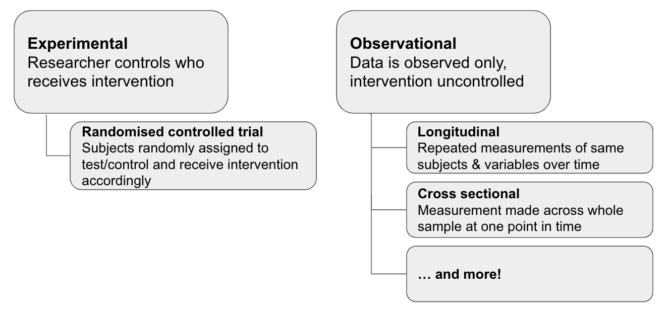
However, due to factors outside the researcher’s control, it is not always possible to run a randomised trial, leading to the class of study we will investigate in this blog post - namely the observational study. In an observational study, the intervention (for example a treatment in the medical case, using a certain product in the OVO case) is not controlled by the researcher, which introduces a source of bias into any conclusions drawn from this data. This can be easily illustrated with the idea of self selection - if you run a medical trial, you may find that the sickest people are more likely to take a particular treatment, however they are also the people most likely to have the worst outcomes without treatment. Therefore any study comparing those treated vs non treated will be biased if the level of patient sickness prior to treatment is not accounted for.
Despite these issues, observational data is often plentiful and we would still like to learn from it, so various mitigation strategies have been developed. One possible approach is to follow a two step procedure:
- Run matching process to create a pseudo-control group from your non-treatment subjects
- Build inference model predicting the outcome of interest, given the treatment assignment and any other explanatory variables
Actually you can run an analysis using either of these steps, but combining them aims to make the analysis “doubly robust" - the idea being that if something is not picked up in one of the steps, the analysis is still protected by the other step. Let’s explore both of these in a bit more detail.
Matching process
The matching step can be motivated by the medical trial example above - in the absence of randomised assignment, individuals with relevant characteristics may be more likely to receive some intervention (“sickness” used above but other important factors in medical case may be things like age, smoking history, etc). These same characteristics may also influence the outcome you’re interested in assessing, in which case the characteristics are said to be “confounding” variables.
The purpose of matching is to sever one of these dependencies (the link to the independent variable) - when we perform a matching process using the confounding variables, we are essentially conditioning on the values of those variables, thereby removing the dependency:

Skipping any maths, the intuition for why this works can be understood from the diagram below - by removing the subjects that don’t have a match in the other group, we’re ensuring that our treatment and control group are as comparable as possible.
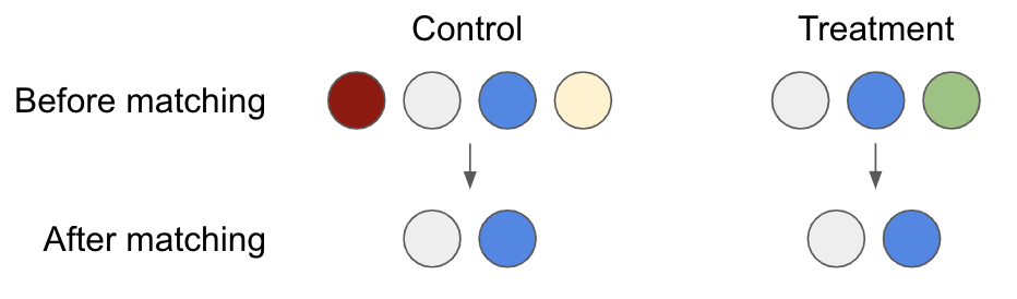
There are a number of different matching processes used for this purpose; Propensity Score Matching (PSM, introduced in 1983) is arguably the most common. In PSM, you build a classification model with treatment/page visit as the target variable and any potential confounding variables as predictors. You then match records based on the propensities predicted by the model (or in the close vicinity of the prediction, known as calliper band matching). Records that are not close to any others in terms of probability are discarded, as illustrated in the diagram above.
The downside to PSM is that it only approximates a randomised controlled trial, whereas the ideal is so-called randomised fully blocked (this means that the control/treatment subpopulations also match on relevant important factors (e.g age, smoking history in medical case) - in a randomised controlled trial, this could be achieved by stratified treatment assignment). One alternative is Coarsened Exact Matching (CEM). Intuitively this is easy to understand - rather than build a predictive model, you match exactly on the potential confounding variables, coarsened/banded to an appropriate degree to avoid a highly punitive match that drops lots of records. This by definition enforces the fully blocked aspect, although the downside is that not all the variables you include will actually be confounding and so you may remove more data than necessary, with no way of illuminating this unlike the PSM case.
Whatever matching methodology is picked, the process is only as good as the data that is available for matching, so there are still limitations. For example a researcher could easily overlook certain variables to include in the matching, or there may be some latent unmeasurable confounding factors. This is a major issue - unlike with a randomised trial, you can never be sure this isn’t the case. With both PSM & CEM there are further caveats around researcher discretion, since both have a number of tunable knobs - for example widening the probability matching band in the PSM case & the degree of coarsening in the CEM case.
Inference model
Once we have our data set up in a causal framework (for example data from a randomised controlled trial or data after applying the matching process above), inference is about trying to identify what the impact of some treatment for an individual is. We generally only observe one of the treated or untreated states for an individual (e.g in the treatment group you only observe the treated state), so it is necessary to estimate the unseen (counterfactual) state.
There are various approaches for this - on the simple side we might interpret the treated/untreated groups directly as the counterfactual for the other, and do a direct calculation between the groups (e.g. some estimate of the mean effect size and an appropriate statistical test).
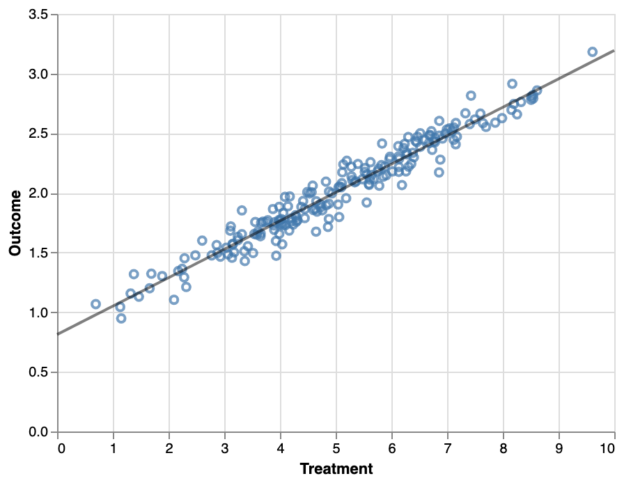
Generally, this is done by building an estimator of the outcome given various control variables, for example using linear or logistic regression. For a simple binary intervention (e.g. has received treatment, has visited page, etc), the model contains the control variables as predictors along with a binary variable indicating the intervention status - the impact of the intervention can then be directly interpreted as the coefficient of the variable. Note that as mentioned above, the modelling step is to make the analysis doubly robust, an alternative approach could be the regression analysis without matching.
Summary
And that’s it! Inference in 2 easy steps ;). Of course, this is just one example approach - in reality this is a vast field and there are many different ways of framing a problem & modelling approaches. Additionally, many problems will have further constraints that are not considered here (for example, what happens when the intervention happens at different time for different people?), but I hope this is illustrative of how you might approach such a situation.
Stay tuned for part 2 where we show how we've applied this to real questions at OVO!
Further reading:
- Causal Inference: What if, Hernán & Robins
- Counterfactuals & Causal Inference, Morgan & Winship, chapters 4 & 5
- MatchIt R package docs & vignette
- CEM R package docs & vignette